In this blog post we will be focusing on MobileNet v1 using Separable Convolutions. Also we will focus on the differences between normal convolutions and separable convolutions and differences between their memory consumptions.

There are basically two types of CNN:

1. Simple Convolutional neural netwroks
2. Depth wise separable convolutional networks

In most of the cases we use simple convolutional networks, but in wide range of cases we require to deploy them into mobile applications, for which we need to reduce the computations. There are majorly two dis-advantages of simple convolutional networks:

1. It contains much more number of parameters, which increases overfitting in most of the cases.
2. They are computationally expensive because of large number of computations and hence cannot be used for mobile applications.

To overcome these advantages, Google proposed two networks namely MobileNet and Xception. In this blog, we will focus on the type of convolutions used in MobileNetv1 i.e depth wise separable convolutional networks. First, we will find how computationally expensive simple convolutional networks are and then move ahead.

Simple Convolutions:

Suppose, we have input data of size PxPxM, where PxP is the image width and image height and M is the number of channels. Also suppose we have N kernels of size KxKxM. After convolution operation is done, the output size will be RxRxN where R is the output image width and height of the image.

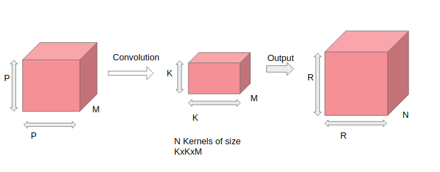
The number of operations performed per convolution will be KxKxM, which is the size of the filter itself. Also, the total number of operations is (Number of operations per convolution)* (RxRxN) = (KxKxM)*(RxRxN).

Depth Wise Separable Convolutions:

It has two major components. The first one is Depth-wise convolution and the second one is Point-wise convolution. We will look into each of them one by one. It is like divide and conquer policy which reduces the cost of computations a lot.

1. Depth-wise convolution

In this type, convolution is applied to a single channel at a time and not like the simple convolutions in which it is done for all the channels together. So here for each convolution,the kernel used is of size K x K x 1. If the number of channels in input image is M, then M such kernels will be used. The output size will be of size R x R x M.

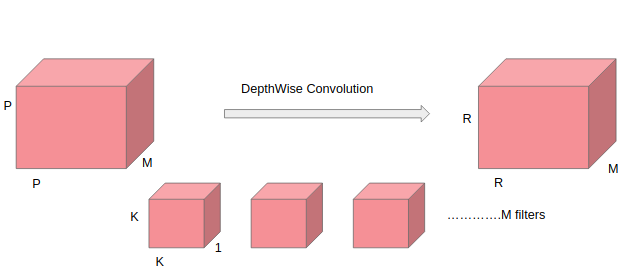
A single convolution would require KxK operations. Since the filter is slided R x R x M, times total cost of operation is RxRxMxKxK.

2. Point-wise convolution

In point-wise operation, a 1 × 1 convolution operation is applied on the M channels. So the filter size for this operation will be 1 x 1 x M. Say we use N such filters, the output size becomes R x R x N.

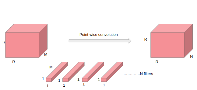
A single point-wise convolution require 1xM operations Since the filter is slided RxR times, total number of multiplications required is (1xM)*(RxR) = MxRxRxN.

Total time complexity for Depth separable convolutions is sum of computations required in depth wise and point wise convolutions which is equal to MxPxPx(RxR+N)

Total complexity for standard convolutions is NxPxPxRxRxM. The chart below shows the comparison in terms of computations between the two types of convolutions.

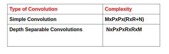
From the below chart we can find that depth wise convolution network performs 100 times lesser multiplications as compared to standard convolutions.

MobileNet v1:

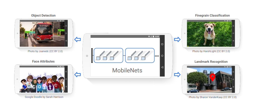
MobileNets are based on a streamlined architecture that uses depthwise separable convolutions to build light weight deep neural networks.In many real world applications such as robotics, self-driving car and augmented reality, the recognition tasks need to be carried out in a timely fashion on a computationally limited platform. This paper describes an efficient network architecture and a set of two hyper-parameters in order to build very small, low latency models that can be easily matched to the design requirements for mobile and embedded vision applications. MobileNet released by Google, is majorly used for mobile applications. The following figure shows the comparison between different netwroks and how MobileNet outperforms it using depth wise separable convolutions.

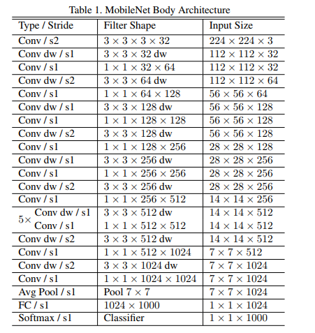
Architecture:

Comparison of the performance between MobileNet and other networks:

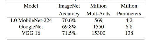
We can see that MobileNet is way much better than other models, in terms of number of parameters, accuracy and in terms of number of computations required. MobileNet outperforms in every aspect.

References:

1. MobileNet